Assignment 4
- Exercise
9.9 (12 marks)
We
use a very simple ontology to make the examples easier:
a.
Horse(x) ⇒ Mammal(x)
Cow(x) ⇒ Mammal(x)
Pig(x) ⇒ Mammal(x)
b.
Offspring(x, y) ∧ Horse(y) ⇒ Horse(x)
c.
Horse(Bluebeard)
d.
Parent(Bluebeard,Charlie)
e. Offspring(x, y) ⇒
Parent(y, x)
Parent(x, y) ⇒
Offspring(y, x)
(Note
we couldn’t do Offspring(x, y) ⇔ Parent(y, x) because that is
not in the form
expected by Generalized Modus Ponens.)
f.
Mammal(x) ⇒ Parent(G(x), x) (here G is a Skolem function).
- Exercise
9.10 a, b (6mark)
This questions deals with the subject of looping in
backward-chaining proofs. A loop is bound to occur whenever a subgoal arises that is a substitution instance of one of
the goals on the stack. Not all loops can be caught this way, of course, otherwise we would have a way to solve the halting
problem.
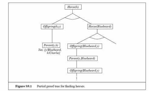
a. The proof tree is shown in Figure S9.1. The
branch with Offspring(Bluebeard, y) and Parent(y,Bluebeard) repeats
indefinitely, so the rest of the proof is never reached.
b. We get an infinite loop because of rule b,
Offspring(x, y) ∧ Horse(y) ⇒ Horse(x). The specific
loop appearing in the figure arises because of the ordering of the clauses—it
would be better to order Horse(Bluebeard) before the rule from b. However, a
loop will occur no matter which way the rules are ordered if the theorem-prover is asked for all solutions.
- Exercise
13.6 (8 marks)
a.
This asks for the probability that Toothache is true.
P(toothache) = 0.108 + 0.012 + 0.016 + 0.064 = 0.2
b.
This asks for the vector of probability values for the random variable Cavity.
It has two values, which we list in the order <true, false>. First add up 0.108 + 0.012 + 0.072 + 0.008 = 0.2. Then we have P(Cavity) = <0.2, 0.8> .
c.
This asks for the vector of probability values for Toothache, given that
Cavity is true.
P(Toothache|cavity) = <(.108 + .012)/0.2, (0.072 + 0.008)/0.2> = <0.6, 0.4>
d.
This asks for the vector of probability values for Cavity, given that
either Toothache or Catch is true. First compute P(toothache ∨catch) = 0.108+0.012+0.016+0.064+ 0.072 + 0.144 = 0.416. Then
P(Cavity|toothache ∨ catch)
=<(0.108 + 0.012 + 0.072)/0.416, (0.016 + 0.064 + 0.144)/0.416>
= <0.4615, 0.5384>
- Exercise
13.8 (6 marks)
We are given the following information:
P(test|disease) = 0.99
P(¬test|¬disease)
= 0.99
P(disease) = 0.0001
and the observation test.
What the patient is concerned about is P(disease|test).
Roughly speaking, the reason it is a good thing that the disease is rare is
that P(disease|test) is proportional
to P(disease), so a lower prior for disease will mean a
lower value for P(disease|test). Roughly
speaking, if 10,000 people take the test, we expect 1 to actually have the
disease, and most likely test positive, while the rest do not have the disease,
but 1% of them (about 100 people) will test positive anyway, so P(disease|test) will be about 1
in 100. More precisely, using the normalization equation from page 428:
P(disease|test)
= P(test|disease)P(disease)
/ (P(test|disease)P(disease)+P(test|¬disease)P(¬disease))
= 0.99×0.0001 / (0.99×0.0001+0.01×0.9999)
= .009804
The moral is that when the disease is much rarer than the
test accuracy, a positive test result does not mean the disease is likely. A
false positive reading remains much more likely. Here is an alternative
exercise along the same lines: A doctor says that an infant who predominantly
turns the head to the right while lying on the back will be right-handed,
and one who turns to the left will be left-handed. Isabella predominantly
turned her head to the left. Given that 90% of the population is right-handed,
what is Isabella’s probability of being right-handed if the test is 90%
accurate? If it is 80% accurate? The reasoning is the
same, and the answer is 50% right-handed if the test is 90% accurate, 69% right-handed
if the test is 80% accurate.
- Exercise
14.1 a, b, c, d (10 marks)
Adding variables to an existing net can be done in two
ways. Formally speaking, one should insert the variables into the variable
ordering and rerun the network construction process from the point where the
first new variable appears. Informally speaking, one never really builds a
network by a strict ordering. Instead, one asks what variables are direct
causes or influences on what other ones, and builds local parent/child graphs that
way. It is usually easy to identify where in such a structure the new variable
goes, but one must be very careful to check for possible induced dependencies
downstream.
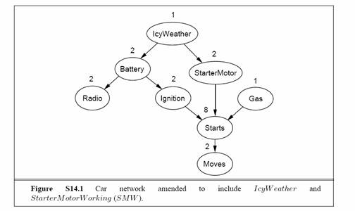
a. IcyWeather
is not caused by any of the car-related variables, so needs no parents.
It directly affects the battery and the starter motor. StarterMotor
is an additional precondition for Starts. The new network is shown
in Figure S14.1.
b. Reasonable probabilities may vary a lot
depending on the kind of car and perhaps the personal experience of the
assessor. The following values indicate the general order of magnitude and
relative values that make sense:
• A
reasonable prior for IcyWeather might be 0.05
(perhaps depending on location and season).
• P(Battery|IcyWeather) = 0.95,
P(Battery|¬IcyWeather) = 0.997.
• P(StarterMotor|IcyWeather) = 0.98,
P(Battery|¬IcyWeather) = 0.999.
• P(Radio|Battery) = 0.9999,
P(Radio|¬Battery) = 0.05.
• P(Ignition|Battery) = 0.998,
P(Ignition|¬Battery) = 0.01.
• P(Gas) = 0.995.
• P(Starts|Ignition, StarterMotor,Gas) = 0.9999, other entries 0.0.
• P(Moves|Starts) = 0.998.
c. With 8 Boolean variables, the joint has 28
− 1 = 255
independent entries.
d. Given the topology shown in Figure S14.1, the
total number of independent CPT entries is 1+2+2+2+2+1+8+2= 20.
- Exercise 14.3 (10marks)
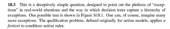
- Exercise 18.3 (4 marks)
- Exercise 18.4 (5 marks)