Introduction

Multithreading enables programmers to speed up their programs by taking advantage of concurrent execution of multiple threads, with each thread assigned to a different CPU core. On the surface, this type of programming may seem easy, but in practice it can be difficult to ensure correctness and to obtain signficant speedup. It's worth learning about multithreading from a parallel computing course and/or from a textbook, such as my Elements of Parallel Computing [1]. These notes are only meant to present some of the features of Julia's support for multithreading, and not a complete course in the subject.

Julia supports two different models for multithreaded programming: loop parallelism with the @threads macro and task parallelism with the Threads.@spawn macro. The latter was announced in July 2019, and is available in Julia 1.3 and higher. These notes were written for Julia 1.5. Upcoming features include adding a foreach function and scheduling options.

These notes will use Julia set fractals to illustrate multithreading. The fractals are pretty, they are easy to compute, and they have a property that makes getting good multithreading performance nontrivial... and then there's the name of the fractals! The core of the calculation is an iteration of the complex-valued function $f(z) = z^2 + c$, where the real and imaginary parts of $z$ are inititialized to coordinates of a pixel in an image and $c$ is another complex number that specifies a particular Julia set. The iterations continue until $|f(z)|>2$ or 255 iterations have completed. The number of iterations can then be mapped to the pixel's color. The Julia function returns an 8 bit integer, given the limited range of values. This function was taken from a Julia Discourse discussion of Julia sets, and was written by Simon Danisch:

function juliaSetPixel(z0, c)
    z = z0
    niter = 255
    for i in 1:niter
        abs2(z)> 4.0 && return (i - 1)%UInt8
        z = z*z + c
    end
    return niter%UInt8
end

juliaSetPixel (generic function with 1 method)

Calculation of one column of the image is computed with the following function:

function calcColumn!(pic, c, n, j)
    x = -2.0 + (j-1)*4.0/(n-1)
    for i in 1:n
        y = -2.0 + (i-1)*4.0/(n-1)
        @inbounds pic[i,j] = juliaSetPixel(x+im*y, c)
    end
    nothing
end

calcColumn! (generic function with 1 method)

where it can be seen that the image has n x n pixels and the range of the coordinates is from -2 to 2. Calculation of the entire fractal is given by:

function juliaSetCalc!(pic, c, n)
    for j in 1:n
        calcColumn!(pic, c, n, j)
    end
    nothing
end

juliaSetCalc! (generic function with 1 method)

More in the next section on why this decomposition into columns has been used. Here is the driver function to generate the fractal:

function juliaSet(x, y, n=1000, method = juliaSetCalc!, extra...)
    c = x + y*im
    pic = Array{UInt8,2}(undef,n,n)
    method(pic, c, n, extra...)
    return pic
end

juliaSet (generic function with 3 methods)

This function allows different parallel versions of the fractal calculation to be passed as a parameter, and the varargs (C programmers will know about this) parameter extra... allows for differences in the number of parameters.

The fractal can be visualized using the heatmap function of the the Plots.jl package. Here is the fractal for $c = -.79 + 0.15i$:

frac = juliaSet(-0.79,0.15)
using Plots
plot(heatmap(1:size(frac,1),1:size(frac,2), frac, color=:Spectral))

Let's run it again to get the execution time:

using BenchmarkTools
@btime juliaSet(-0.79,0.15)

41.115 ms (2 allocations: 976.70 KiB)

;

Parallel Execution

There are three steps to parallelization. The first is to identify a decomposition into tasks that could be computed concurrently. Here it's clear that calculation of each pixel can be done independently of any other pixel. This means that we could have n x n tasks executing in parallel. The second step is to figure out how many tasks are appropriate for the parallel computer we will be using. Current multicore processors have only a small number (at least 2 up to 12 or so) of cores, so n x n tasks is too many. If the number of tasks is too large compared to the number of threads, then the overhead of scheduling them will slow down the computation. A simple way to aggregate tasks is to have one task per column, which has the advantage over rows that Julia stores 2D arrays in column-major order. If this is still too many tasks, then each task can have a contiguous block of columns. The third step is to figure out how to map tasks to threads. We'll look at two ways of doing this, using the @threads macro and the Threads.@spawn macro.

Loop Parallelization with @threads

The @threads macro, when applied to a for loop, decomposes the iterations into contiguous blocks, one for each thread. For instance, if there are 9 iterations and 3 threads, then thread 1 gets iterations 1-3, thread 2 gets iterations 4-6, and thread 3 get iterations 7-9. (As an aside, one nice benefit of working with an open-source language is that you can look up the source code for any language feature to get a better understanding than the documentation provides. So, if you want to understand better how the @threads macro works, have a look at the source code!). This way of mapping tasks (here a task is an iteration of the loop) to threads is called static scheduling, where there is one task per thread, and the mapping is done at compile time. Julia 1.5 includes a schedule argument to choose among scheduling policies, but only currently supports the static schedule just described.

Getting back to our fractal, we can simply add the @threads macro to the for loop in JuliaSetCalc!:

import Base.Threads.@threads
function juliaSetCalcThread!(pic, c, n)
    @threads for j in 1:n
        calcColumn!(pic, c, n, j)
    end
    nothing
end

juliaSetCalcThread! (generic function with 1 method)

with the result that each thread will calculate a contiguous block of columns. Before running a multithreaded Julia program the number of threads needs to be set. This can be done by changing a setting in the IDE, such as the Julia: Num Threads option in VSCode's settings, and then rebooting the IDE. The number of threads can also be set when you're launching Julia from the command line, either using the -t command line arguments, or using the JULIA_NUM_THREADS environment variable. This document was created in Julia on a CPU with more than 4 cores, and was launched with:

$ julia -t 4

You can verify the number of threads using:

Threads.nthreads()

4

First, we want to verify that the fractal is correct:

fracP1 = juliaSet(-0.79,0.15,1000,juliaSetCalcThread!)
fracP1 == frac

true

Let's see how much faster it is:

@btime juliaSet(-0.79,0.15,1000,juliaSetCalcThread!)

17.308 ms (26 allocations: 979.80 KiB)

;

You should notice that we're not getting a speedup of 4 here, more like a value closer to 2. What happened? I modified the calcColumn() function to keep track of the number of iterations for each thread (recall that this is stored in the pic array, and determines the color of the pixel), and generated the following graph:

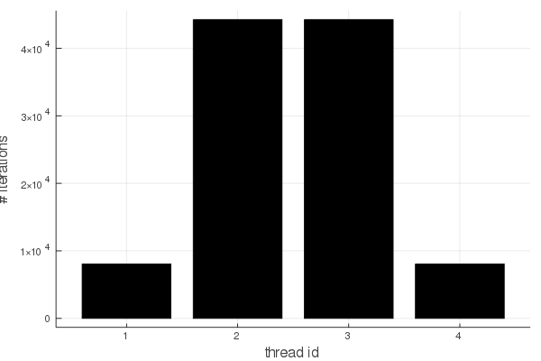
This shows that threads 2 and 3 have the large majority of the iterations, and illustrates nicely why the speedup is only a bit better than 2. Have a look at the fractal picture again, and recall that each thread gets 1/4 of the columns. The further the color is away from red in the spectrum, the more iterations are required. Therefore it can easily be seen that the middle of the image takes more work to compute than the edges, and therefore threads 1 and 4 will have less work to do.

Parallel fractals are a nice example of load imbalance. The static block assignment used by @threads is fine if each task takes the same amount of time. If the runtime of the tasks varies, dynamic scheduling is required to balance the load of the threads. This can be done using Threads.@spawn.

Dynamic Task Scheduling with Threads.@spawn

The Threads.@spawn macro creates a task that is submitted to a scheduler for execution on a thread. The programming model was inspired by previous task based models, such as Cilk. It is also similar to Java's Fork-Join framework. The Threads.@spawn macro is suited to a recursive divide-and-conquer approach. A good example is merge sort, where the problem is divided into sorting each half, then merging them together, as the following pseudocode illustrates:

mergeSort(a,1,n)
    mid = (1+n)/2
    mergeSort(a,1,mid)
    mergeSort(a,mid+1,n)
    merge(a,1,mid,n) # merge a[1:mid] with a[mid+1:n]
end

The two recursive calls can be make concurrently, so the first call can be forked into a new task. When the current task returns from its recursive call, it waits (joins) until the forked task completes:

mergeSortP(a,1,n)
    mid = (1+n)/2
    fork mergeSortP(a,1,mid)
    mergeSort(a,mid+1,n)
    join
    merge(a,1,mid,n) # merge a[1:mid] with a[mid+1:n]
end

This way, the current task and the spawned task can run in parallel. It's important to understand that forking does not create a new thread, but that it creates a new task that can run on another thread. In Julia the fork is done with Threads.@spawn and the join is done with fetch() to get the return value or wait() if there is no return value. A simple implementation of mergesort is given in the blog post announcing this programming model. As an aside, one can get even better performance by parallelizing the merge [1]. Each time a task is created, it is sent to the scheduler for assignment to a thread.

Getting back to our fractal, we can use a divide-and-conquer approach, by recursively dividing up the columns:

function juliaSetCalcR!(pic, c, n, lo=1, hi=n)
     if hi > lo
         mid = (lo+hi)>>>1
         finish = Threads.@spawn juliaSetCalcR!(pic, c, n, lo, mid)
         juliaSetCalcR!(pic, c, n, mid+1, hi)
         wait(finish)
         return
     end
     calcColumn!(pic, c, n, lo)
end

One of the recursive calls has been spawned into a new task, and the finish handle is used to wait for its completion. This function will create a task for each column, which may cause the scheduler to work too hard, adding to the execution time. A better version stops the recursion at a given cutoff, which is calculated based in the number of columns and the number of tasks desired:

function juliaSetCalcRecSpawn!(pic, c, n, lo=1, hi=n, ntasks=16)
    if hi - lo > n/ntasks-1
        mid = (lo+hi)>>>1
        finish = Threads.@spawn juliaSetCalcRecSpawn!(pic, c, n, lo, mid, ntasks)
        juliaSetCalcRecSpawn!(pic, c, n, mid+1, hi, ntasks)
        wait(finish)
        return
    end
    for j in lo:hi
        calcColumn!(pic, c, n, j)
    end
    nothing
end

juliaSetCalcRecSpawn! (generic function with 4 methods)

The recursion stops at n/ntasks columns, which will create fewer tasks than our original version. For instance, in our examples we have 1000 columns, so we'll have 16 tasks with 62 or 63 columns each. Let's test the function:

fracP2 = juliaSet(-0.79,0.15,1000,juliaSetCalcRecSpawn!)
fracP2 == frac

true

Let's see how much faster it is:

@btime juliaSet(-0.79,0.15,1000,juliaSetCalcRecSpawn!)

10.593 ms (143 allocations: 994.77 KiB)

;

This speedup is close to 4, which means we've done much better than with the static scheduling of @threads. As in the previous section, we can modify calcColumn() to keep track of the number of iterations per thread:

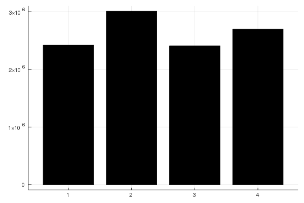
Now we see that each thread gets roughly the same amount of work. We can also look at the mapping of columns to threads by modifying juliaSetCalcRecSpawn!() to store the thread id for each column, giving:

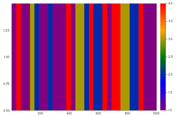
where thread 1 is purple, thread 2 is blue, thread 3 is greenish, and thread 4 is red. This is a much different mapping than the 4 contiguous blocks used by @threads. The mapping is created dynamically by the scheduler, which balances the work among the threads. Note that since the mapping is dynamic, it won't be exactly the same each time the program is run. If we run the program again, we get:

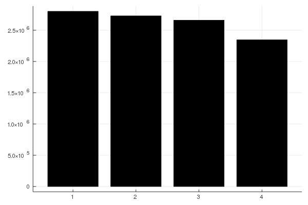
The work is still roughly balanced, but not exactly in the same way as in the first run. The result is close to the same runtime in both cases. It's worthwhile to play with the ntasks parameter to see how it affects the runtime. At one extreme, choosing ntasks=4 will give the same result as the static assignment of @threads, and performance will improve as ntasks is increased, but not necessarily uniformly. What happens if ntask is very large (close to n)?

Final Thoughts

Julia's support for multithreaded programming is continually improving. Right how it provides static loop parallelism and dynamic task-based parallelism, which can cover many cases where pararallelization is called for. This discussion has left out the important topic of read/write conflict of multiple threads, leading to race conditions. In our fractal example, each thread works on its own portion of the image. In general, however, it is very common to have multiple threads access the same memory locations, whether by design or by accident. Julia provides locks and atomic operations to avoid race conditions when shared access is required.

Before embarking on parallelization, it's worth reflecting on whether you need to parallelize. The fractal example was chosen for pedagogical reasons, and serial execution times are so fast that in practice you wouldn't need to parallelize the computation of a Julia set. If your program is too slow, optimize single-threaded performance before trying to change your program to run on multiple threads. Julia's documentation provides some tips on improving performance.

---