Introduction

* LightGraphs has been replaced by the Graphs package.

The biggest challenge with multithreaded programming is dealing with race conditions that arise from multiple threads performing reads and writes to a location in memory. My previous Notes on Multithreading in Julia avoided this problem by calculating a fractal with multiple threads, where each thread worked on distinct elements of a two-dimensional array. In most cases, multithreaded programs can't avoid dealing with race conditions as easily, and some kind of synchronization must be used to control access to shared memory locations. A common way to do this is to protect access to shared memory locations using locks. While this is a standard technique in concurrent programs, locks can lead to poor performance in shared memory parallel programs. Lock-free techniques use lower level synchronization with atomic operations to deliver better multithreading performance.

My goal in this document is to demonstrate the use of atomics in a parallel implementation of the Bellman-Ford algorithm for solving the all-pairs shortest path problem. A detailed discussion of parallel all-pairs shortest path algorithms is given in Chapter 6 of my book, Elements of Parallel Computing [1]. This book also discusses race conditions and lock-free programming using atomics.

Sequential Bellman-Ford

The single-source-shortest-path (SSSP) problem is to find the shortest path from a single vertex to all other vertices in a weighted directed graph. Here I will focus only on finding the weights of the shortest paths. We will need some way to represent a graph in Julia. A good data structure is provided in the LightGraphs and SimpleWeightedGraphs packages Here's a version of the Bellman-Ford algorith that uses a queue to store vertices (see Elements of Parallel Computing [1], Chapter 6):

using LightGraphs, SimpleWeightedGraphs, DataStructures
# Relax neighbours of i
function relax(g, D, List, InList, i)
    @inbounds for j in neighbors(g,i)
       # weights[j,i] gives weight of edge i->j
       if D[j] > D[i] + g.weights[j,i]
          D[j] = D[i] + g.weights[j,i]
          if(!InList[j])
             push!(List, j)
             InList[j] = true
          end
       end
    end
 end
 
 function ssspbfgraph(g, source)
    n = nv(g)
    m = ne(g)
 
    # Circular buffer to hold FIFO list
    List = CircularBuffer{Int}(n)
    # Sparse representation of list
    InList = zeros(Bool,n)
 
    D = fill(typemax(eltype(g.weights)),n)
    D[source] = zero(eltype(g.weights))
    push!(List, source)
    InList[source] = true
 
    while length(List) > 0
       i = popfirst!(List)
       InList[i] = false
       relax(g, D, List, InList, i)
    end
    return D
 end

ssspbfgraph (generic function with 1 method)

The queue is represented twice: as a circular buffer List and as a boolean array inList. The second representation, in which the presence of vertex i in the queue is indicated by setting position i in the boolean array, allows the program to quickly determine whether a vertex is in the queue. The queue is initialized with the source vertex. The weights of the shortest paths are stored in the distance array D, which is initialized to "infinity" (the maximum value allowed by the data type used to represent weights), except to zero for the position of the source vertex.

The algorithm proceeds iteratively by removing a vertex from the queue, "relaxing" edges out from this vertex, until the queue is empty. Edges i->j are relaxed by replacing D[j] (the current distance to j) with D[i] plus the weight of edge i->j if this reduces the value of D[j]. If D[j] is updated, then j is added to the queue (if it is not already there). Note that adding to the queue involves two operations: pushing to the queue and setting the jth element of inList.

A graph needs to be constructed to test the performance of the sequential and parallel SSSP algorithms. Here we'll use a Kronecker graph, which is a type of random graph used in the Graph 500 benchmark. I modified the Kronecker function from the LightGraphs package so that it generates a SimpleWeightedDiGraph. All this required was changing the graph type and the call to add_edge to add_edge!(g, s, d, rand(rng,1)[1]). I also skipped sef-edges.

using Random:
    AbstractRNG, MersenneTwister, randperm, seed!, shuffle!
using Statistics: mean

using LightGraphs:
    getRNG, sample!

using LightGraphs, SimpleWeightedGraphs
"""
    kronecker(SCALE, edgefactor, A=0.57, B=0.19, C=0.19; seed=-1)
Generate a directed [Kronecker graph](https://en.wikipedia.org/wiki/Kronecker_graph)
with the default Graph500 parameters.
###
References
- http://www.graph500.org/specifications#alg:generator

Modified by Eric Aubanel, March 2020, add create weighted
graph with random weights between 0 and 1. Skips self-edges
"""
function kroneckerwt(SCALE, edgefactor, A=0.57, B=0.19, C=0.19; seed::Int=-1)
    N = 2^SCALE
    M = edgefactor * N
    ij = ones(Int, M, 2)
    ab = A + B
    c_norm = C / (1 - (A + B))
    a_norm = A / (A + B)
    rng = getRNG(seed)

    for ib = 1:SCALE
        ii_bit = rand(rng, M) .> (ab)  # bitarray
        jj_bit = rand(rng, M) .> (c_norm .* (ii_bit) + a_norm .* .!(ii_bit))
        ij .+= 2^(ib - 1) .* (hcat(ii_bit, jj_bit))
    end

    p = randperm(rng, N)
    ij = p[ij]

    p = randperm(rng, M)
    ij = ij[p, :]

    g = SimpleWeightedDiGraph(N)
    for (s, d) in zip(@view(ij[:, 1]), @view(ij[:, 2]))
        if s == d
            continue
        end
        add_edge!(g, s, d, rand(rng,1)[1])
    end
    return g
end

Main.##WeaveSandBox#253.kroneckerwt

To ensure that the same graph is used in the sequential and parallel runs, a graph was generated (with g = kroneckerwt(17,16)) and saved to a file with savegraph( "kroneckerwt17_16.lgz", g). The loadgraph function is used to load the graph (note the second parameter that specifies that it's a simple weighted graph):

g = loadgraph("kroneckerwt17_16.lgz",SWGFormat())

{131072, 1942691} directed simple Int64 graph with Float64 weights

This graph has 2^17 vertices and up to 16 x 2^17 edges (fewer since self-edges skipped). We need to pick a source vertex to run ssspbfgraph(), and one that has at least one out-edge (otherwise there will be no paths at all!). Here's a run with source vertex 2, on a computer with two 24 core Intel® Xeon® Platinum 8168 processors:

using BenchmarkTools
@btime Ds = ssspbfgraph(g,2)

371.722 ms (7 allocations: 2.13 MiB)
131072-element Array{Float64,1}:
 Inf
  0.0
 Inf
 Inf
  0.7616966902321791
  0.6578596382832484
 Inf
 Inf
  0.12751008318592016
  0.09061644820757642
  ⋮
 Inf
  0.0991263824375701
  0.8030456717521828
 Inf
  0.040778978033212177
 Inf
 Inf
 Inf
  0.12435354711105284

Note that the distance from vertex 2 to itself is zero, and some vertices are unreachable from vertex 2, as shown by a distance of Inf.

Parallel Bellman-Ford

Designing a parallel algoritm involves identifying tasks that can be executed in parallel. In the case of Bellman-Ford we can choose to process all of the vertices in the queue at each iteration. There's no requirement to use a queue in a Bellman-Ford implementation; it just works well for the sequential program. Processing all the vertices in the list in parallel promises to deliver some speedup at the cost of more relaxations than the sequential program.

We need to choose between a single shared list or a separate list for each thread. A shared list would require synchronizing updates; as these would be constantly occuring there would be significant overhead. A better solution is to have each thread add vertices to its own list, then have all threads copy their vertices to a shared list.

Atomic Type and Operations

We'll still need to use synchronization for updates of the D array, however. We need updates to be atomic, that is the low-level operations needed to update an element of D can only be done by one thread at a time, wihout being interrupted by another thread. This can be done by using Julia's atomic type: D = [Atomic{T}(typemax(T)) for k = 1:n], where T is the same type that was used in the sequential program. This statement creates an array of of atomics and initializes each element to the maximum value available in type T. Note that atomic types are only available for boolean, integer and float types. The parallel relax function will use two atomic operations: atomic_min! and atomic_cas!. We'll look at each in turn, but first let's see what happens with a nonatomic min. We have 8 threads:

using Base.Threads
nthreads()

8

but we'll only use 2:

function nonatomicMin()
   x = Inf
   @threads for i in 1:2
       (i*100.0 < x) ? (x=i*100.0) : ()
   end
   return x
end

nonatomicMin (generic function with 1 method)

This function has two threads compare 100.0 and 200.0, respectively, with x, and replace x if the condition is met. We might expect 100.0 to be returned:

nonatomicMin()

100.0

but if we run this function many times, we can see that sometimes 200 is returned:

for i in 1:10000
   r = nonatomicMin()
   if r != 100.0
      println(i,": ",r)
   end
end

1416: 200.0
2443: 200.0
4048: 200.0
7892: 200.0
8915: 200.0

This is an example of non-deterministic behaviour resulting from a race condition for x: both threads are reading and writing to x without synchronization. The problem is that the conditional statement is not atomic, so for instance, both threads could perform i*100.0 < x before either thread updates 'x', with the final value of x determined by the order of the execution of x=i*100.0. When thread 1 performs the write first, thread 2 will overwrite x with 200.0. To avoid this race condition, we need to make the entire (i*100.0 < x) ? (x=i*100.0) : () operation atomic, so that only one thread at a time reads and writes to x.

atomic_min!(x, val) stores the minimum of x and val in x atomically and returns the old value of x:

x = Atomic{Float64}(typemax(Float64))
atomic_min!(x, 100.0)

Inf

atomic_min! has returned the old value of x. Here is the new value of x, where the x[] notation is needed to atomically load the value of x:

x[]

100.0

Let's return to our 2 thread example:

function atomicMin()
   x = Atomic{Float64}(typemax(Float64))
   @threads for i in 1:2
       atomic_min!(x, i*100.0)
   end
   return x[]
end
for i in 1:10000
   r = atomicMin()
   if r != 100.0
      println(i,": ",r)
   end
end

There is no output, which means all return values were 100.0. Note that this in itself is not a guarantee that there is no race condition. It's the guarantee provided by atomic_min!() that does this. Next, let's look at the following function:

function nonatomicCAS()
   x = 0
   r = zeros(Int, 2) 
   @threads for i in 1:2
       if x == 0
           x = 1
           r[i] = 1
       end
   end
   return r
end

nonatomicCAS (generic function with 1 method)

The intent is to have only 1 thread set an element of r to 1:

nonatomicCAS()

2-element Array{Int64,1}:
 0
 1

However, here again we have a race condition with x:

for i in 1:10000
   r = nonatomicCAS()
   if r[1] == 1 && r[2] == 1
      println(i,": ",r[1],", ",r[2])
   end
end

2534: 1, 1
2897: 1, 1
7447: 1, 1
8216: 1, 1
8825: 1, 1

in the cases when both elements of r are set to 1, each thread has evaluated x==0 before either thread has done x = 1. To avoid this we need to make the comparison and update of x atomic.

The compare-and-swap (also called compare-and-set) is a fundamental atomic operation that many processors implement at the machine level, and that can be used to build other atomic operations. atomic_cas!(x, cmp, newVal) compares x with cmp; if they are equal, newVal is written to x; if not, x is unmodified; finally, the old value of x is returned; all this takes place atomically.

x = Atomic{Int}(0)
atomic_cas!(x,0,1)

0

atomic_cas! returns the old value and x has been set to 1:

x[]

1

Now let's return to our 2-thread example with this function:

function atomicCAS()
   x = Atomic{Int}(0)
   r = zeros(Int, 2) 
   @threads for i in 1:2
       if atomic_cas!(x,0,1) == 0
           r[i] = 1
       end
   end
   return r
end
for i in 1:10000
   r = atomicCAS()
   if r[1] == 1 && r[2] == 1
      println(i,": ",r[1],", ",r[2])
   end
end

No output. The race condition has been removed, since the comparison and update are atomic, and only 1 thread will encounter a value of 0 for x, so only one element of r will be set to 1.

Parallel Implementation

Let's start with ssspbfpargraph:

function ssspbfpargraph(g, source)
   n = nv(g)
   m = ne(g)

   # Vertex list
   List = Array{Int64,1}(undef,n)
   nt = nthreads()
   # Per thread vertex list buffers; will grow if too small
   subList = [similar(List, 10) for i = 1:nt]
   vperthread = zeros(Int64,nt) # Per thread vertex count

   T = eltype(g.weights)
   D = [Atomic{T}(typemax(T)) for k = 1:n]
   InList = [Atomic{Int}(0) for k = 1:n]

   D[source][] = zero(T)
   List[1] = source
   nverts = 1 # no. of vertices in list

   while nverts > 0
      relax(g, D, subList, List, InList, vperthread, nverts)
      # write thread private vertices to shared List
      start = cumsum(vperthread)
      nverts = start[nt]
      start -= vperthread # exclusive prefix sum
      @threads for i = 1:nt
         copyVerts!(List, InList, subList[i], start[i], vperthread[i])
      end
      vperthread .= 0
   end
   return D
end

ssspbfpargraph (generic function with 1 method)

A partially filled array for each thread called subList is allocated. These are initially of length 10, but the relax function will grow them if necessary. We also will keep track of the number of vertices in each sublist, in vperthread. Note that there are two atomic arrays, D and inList. We'll use the second one to avoid storing a vertex more than once in List. Each iteration of the while loop relaxes edges from all vertices in List (recall the sequential while loop iteration only relaxed edges from a single vertex). When relax returns, subList will contain a list of vertices produced by edge thread's relaxations, and vperthread will contain the count of vertices in each sublist. Each thread will copy its vertices to List, so it needs to know where to begin writing. The cumulative sum of vperthread (cumsum in Julia, also know as inclusive prefix sum) will give us the total number of vertices to be written, and almost gives the starting point for each thread. We just need to subtract each thread's vertex sum from the cumulative sum, to give the exclusive prefix sum. For instance, if vperthread = {2,5,4}, the exclusive prefix sum gives start={0,2,7}, which would mean that thread 1 would start writing at index 1, thread 2 at index 3, and thread 3 at index 8 (recall Julia's 1-based indexing!). The parallel (with @threads) loop has each thread copy one of the sublists to List, using the copyVerts function.

function copyVerts!(List, InList, sub, start, nper)
   for i in 1:nper
     InList[sub[i]][] = 0
     List[start+i] = sub[i]
   end
end

copyVerts! (generic function with 1 method)

Note that this function also sets the corresponding element of inList to zero for each vertex copied; this resets inList to all zeros so that it's ready for its next use in the relax function.

# relax neighbours of all vertices in list
function relax(g, D, subList, List, InList, vperthread, nverts)
   #show(List[1:nverts])
   @threads for i in List[1:nverts]
      @inbounds for j in neighbors(g,i)
         # weights[j,i] gives weight of edge i->j
         # atomic_min returns old value
         if atomic_min!(D[j], D[i][] + g.weights[j,i]) > D[j][]
            # atomic to avoid duplicates, then add to thread's list
            # atomic_cas returns old value
            if(atomic_cas!(InList[j],0,1) === 0)
               id = threadid()
               listSize = length(subList[id])
               listSize <= vperthread[id] && resize!(subList[id], 2*listSize)
               vperthread[id] += 1
               subList[id][vperthread[id]] = j
            end
         end
      end
   end
end

relax (generic function with 2 methods)

The relax function iterates through all vertices in List, with each thread assigned a block of iterations. If atomic_min() finds a new minimum for D[j], the old version will be greater than D[j] and atomic_cas() is called to determine whether vertex j is already in the list. Use of an atomic min function ensures that only one thread can update D[j] at a time. Use of the atomic compare-and-swap ensures that only one thread can put j in its list. If vertex j needs to be added to a thread's sublist, but the sublist is full, then it is resized.

Note that even though the atomic_min! is atomic and the access D[j][] is atomic, the entire comparison atomic_min!(D[j], D[i][] + g.weights[j,i]) > D[j][] is not. This means that this comparison could be true even if D[j] is not updated. Consider the following operations, with the precondition that D[j][] has the value 0.5:

1. Thread 1 does not reduce the value, and atomic_min!() returns 0.5

2. Next, thread 2 reduces the value of D[j], say from from 0.5 to 0.4, so atomic_min!() also returns 0.5, and D[j] is now 0.4

3. Next, thread 1 makes the comparison with D[j], which is true, since 0.5 > 0.4

4. Next, thread 2 makes the comparison with D[j], which is also true.

Is it a problem that thread 1 proceeded to the atomic_cas!(), even though it didn't update D[j]? No, it isn't. The behaviour the parallel loop relies on is that if one or more threads update D[j], then j should be added to only one thread's sublist. That is what the atomic_cas! accomplishes. In the interleaving given above, only 1 thread will enter the inner if and add 'j' to it's sublist; we don't care which thread does so.

Let's test our program using 8 threads:

nthreads()

8

Ds = ssspbfgraph(g,2)
Dp = ssspbfpargraph(g,2);
DD = similar(Ds,length(Ds))
for i in 1:length(Ds)
        if Ds[i] == Inf && Dp[i][] == Inf
                DD[i] = 0.0
        else
                DD[i] = Dp[i][] - Ds[i]
        end
end
sumdiff = sum(DD)

0.0

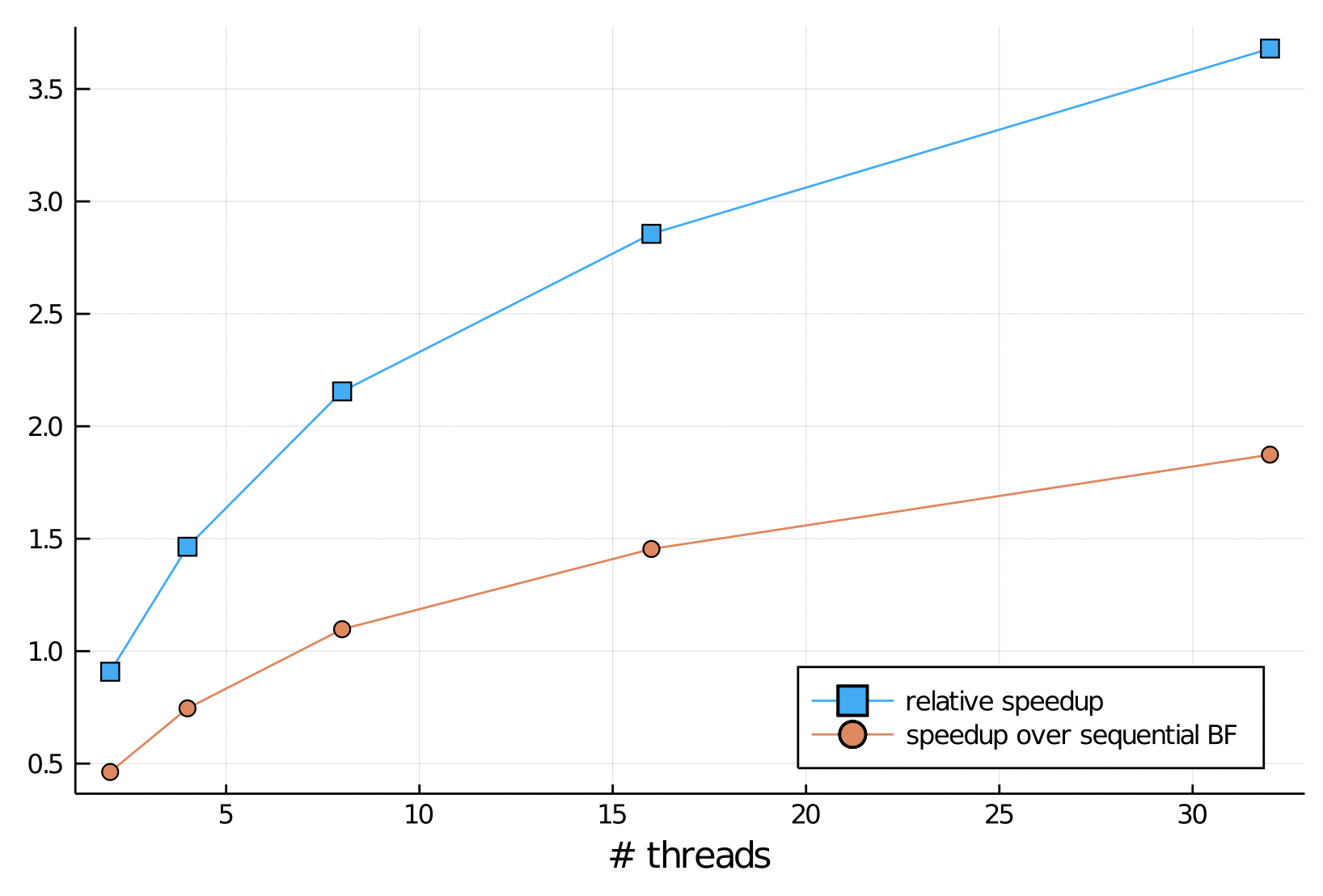
The performance of our parallel Bellman Ford is shown in the two speedup curves below. The blue curve shows the speedup relative to a run with 1 thread. Note that the the program slows down going from 1 to 2 threads, but then improves modestly up to 32 threads. The orange curve shows that speedup compared to the sequential program is only obtained for 8 threads or more. performance of our parallel program is limited by the number of vertices in the list at each call to relax; the longer the list, the greater the work that each thread has, which offsets the parallel overhead. This overhead includes extra relaxations arising from processing all vertices in each iteration, copying from the sublists to the shared list and the cost of the atomic functions. Graphs with larger average vertex degrees will tend to give better performance, since they have longers lists (more edges per vertex), but this will vary with the choice of source vertex.

Final Thoughts

One of the main challenges of shared memory parallel programming is managing access to shared memory to eliminate race conditions. Two basic approaches were illustrated in this example: having threads write to separate memory locations, then merge their results in parallel (subList and List in this program), and synchronizing access using atomic operations.

---