Getting started

• Make a directory ~/cs2613/labs/L21
• Download timeit.m, and put it in your newly created directory

Fibonacci using a constant amount of storage.

As a general principle we may want to reduce the amount of storage used so that it doesn't depend on the input. This way we are not vulnerable to e.g. a bad input crashing our interpreter by running out of memory. We can improve tabfib by observing that we never look more than 2 back in the table. Fill in each blank in the following with one variable (remember, ret is a variable too).

function ret = abfib(n)
  a = 0;
  b = 1;
  for i=0:n
    ret = _ ;
    a = _ ;
    b = _  + b ;
  endfor
endfunction

%!assert (abfib(0) == 0);
%!assert (abfib(1) == 1);
%!assert (abfib(2) == 1);
%!assert (abfib(3) == 2);
%!assert (abfib(4) == 3);
%!assert (abfib(5) == 5);

• This algorithm is quite tricky. To understand how to fill in the blanks
  • what happens for n==0 (first blank)
  • what happens for n==1 (second blank)
  • in loop repetition i, b is assigned to (i+2)nd Fibonacci number.
• Check the change in performance with the following. Although not as spectacular as repacing recursion (in Octave), there should be a noticable speedup.

function bench2
  timeit(10000,@tabfib, 42)
  timeit(10000,@abfib, 42)
endfunction

Fibonaccci as matrix multiplication

The following is a well known identity about the Fibonacci numbers F(i).

[ 1, 1;
  1, 0 ]^n = [ F(n+1), F(n);
               F(n),   F(n-1) ]

This can be proven by induction; the key step is to consider the matrix product

 [ F(n+1), F(n);   F(n),   F(n-1) ] * [ 1, 1; 1, 0 ]

Since matrix exponentiation is built-in to octave, this is particularly easy to implement the formula above in octave

Save the following as ~/cs2613/labs/L21/matfib.m, fill in the two matrix operations needed to complete the algorithm

function ret = matfib(n)
  A = [1,1; 1,0];


endfunction

%!assert (matfib(0) == 0);
%!assert (matfib(1) == 1);
%!assert (matfib(2) == 1);
%!assert (matfib(3) == 2);
%!assert (matfib(4) == 3);
%!assert (matfib(5) == 5);
%!assert (matfib(6) == 8);
%!assert (matfib(25) == 75025);

We can expect the second Fibonacci implementation to be faster for two distinct reasons

• It's possible to compute matrix powers rather quickly (O(log n) compared O(n)), and since the fast algorithm is also simple, we can hope that octave implements it. Since the source to octave is available, we could actually check this.

• Octave is interpreted, so loops are generally slower than matrix operations (which can be done in a single call to an optimized library). This general strategy is called vectorization, and applies in a variety of languages, usually for numerical computations. In particular most PC hardware supports some kind of hardware vector facility.

• For the following, you will need either your solutions from last time, or to download timeit.m and tabfib.m. Note that the code here assumes the repetitions come first for timeit, as expected by the version for this lab.

function bench3
  timeit(10000, @tabfib, 42)
  timeit(10000, @matfib, 42)
endfunction

Questions for your journal

• How much speedup do you see from the matrix multiplication trick?

Broadcasting

In Octave we can multiply every element of a matrix by a scalar using the .* operator

A=[1,2,3;
   4,5,6];
B=A.*2

In general .* supports any two arguments of the same size.

C=A .* [2,2,2; 2,2,2]

It turns out these are actually the same operation, since Octave converts the first into the second via broadcasting

Quoting from the Octave docs, for element-wise binary operators and functions

The rule is that corresponding array dimensions must either be equal, or one of them must be 1.

In the case where one if the dimensions is 1, the smaller matrix is tiled to match the dimensions of the larger matrix.

Here's another example you can try.

x = [1 2 3;
     4 5 6;
     7 8 9];

y = [10 20 30];

x + y

Reshaping arrays

One potentially surprising aspect of Octave arrays is that the number of dimensions is independent from the number of elements. We can add as many dimensions as we like, as long as the only possible index in those dimensions is 1. This can be particularly useful when trying to broadcast with higher dimensional arrays.

     ones(3,3,3) .* reshape([1,2,3],[1,1,3])
     ones(3,3,3) .* reshape([1,2,3],[1,3,1])

Scaling layers of arrays

Complete the following function. You may want to copy the definitions of A and B into the REPL to understand the use of cat.

## usage: scale_layers(array, weights)
##
## multiply each layer of a 3D array by the corresponding weight
function out = scale_layers(array, weights)
  out =
endfunction

%!test
%! onez = ones(3,3);
%! A=cat(3,onez, 2*onez, 3*onez);
%! B=cat(3,onez, 6*onez, 15*onez);
%! assert(scale_layers(A,[1;3;5]),B)

Scaling a colour channel

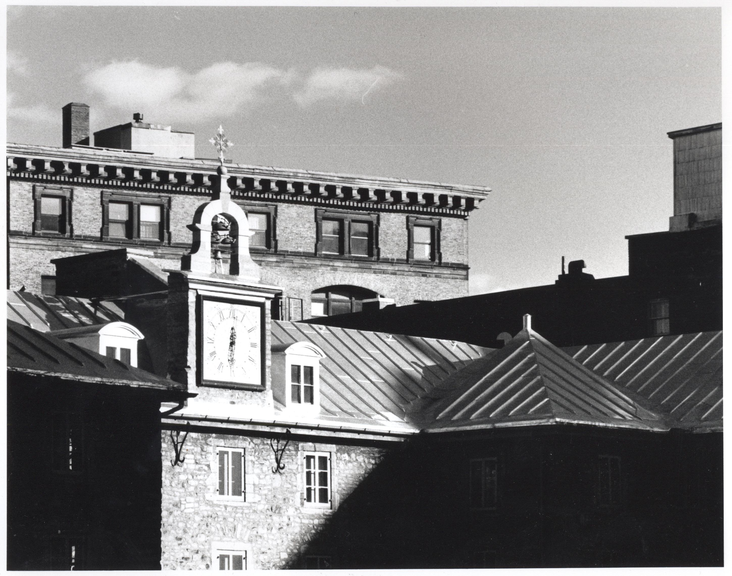
Save the image above left as ~/cs2613/labs/L21/paris.jpg (make sure you get the full resolution image, and not the thumbnail).

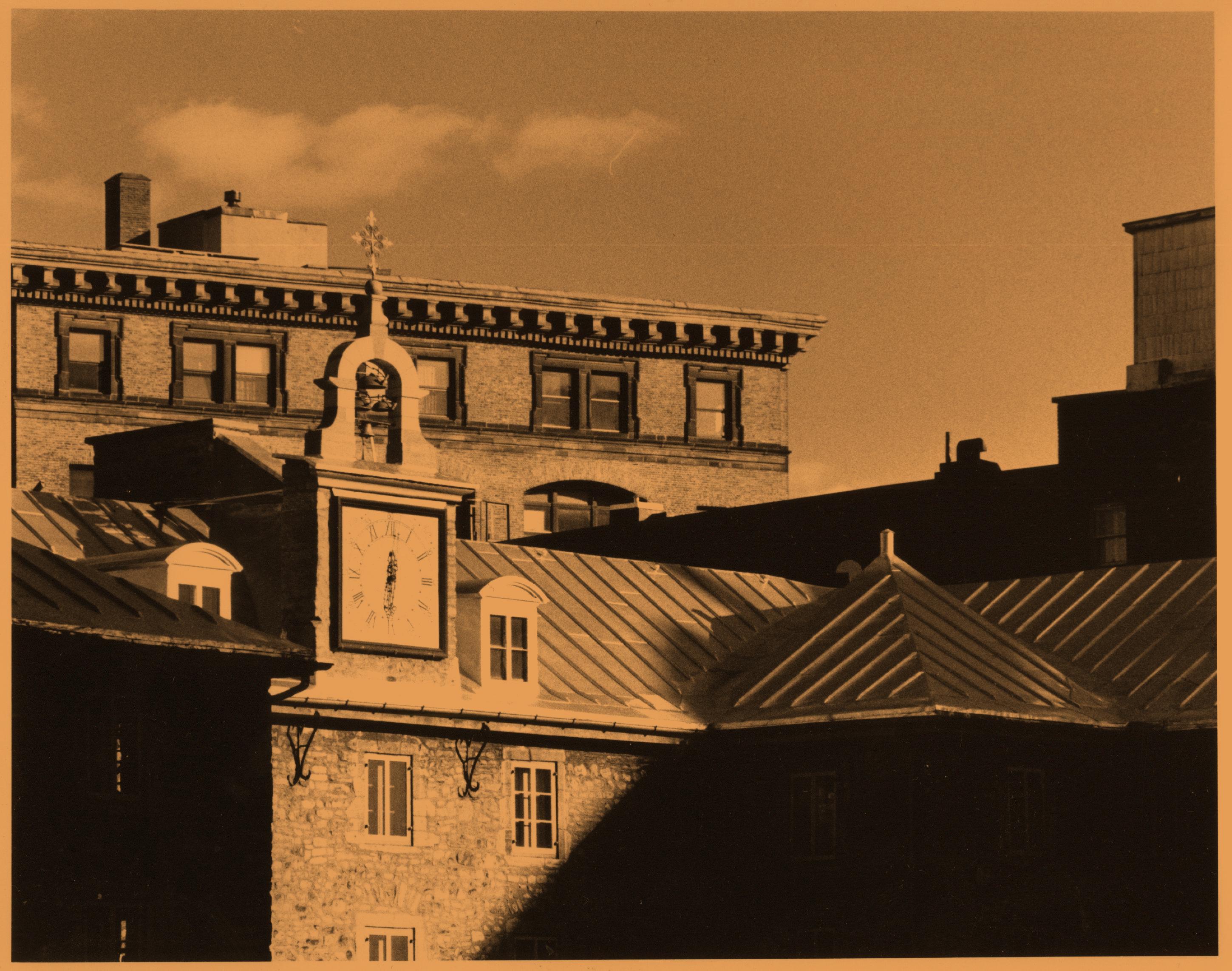
Run the following demo code; you can change the weight vector for different colourization.

paris=imread("paris.jpg");
sepia=scale_layers(paris,[0.9,0.62,0.34]);
imshow(sepia);

You should get something like the following

Before next lab