Before the lab
Read
Either for creative reasons, or as part of a more complex image processing task, it is common to convert images to monochrome.
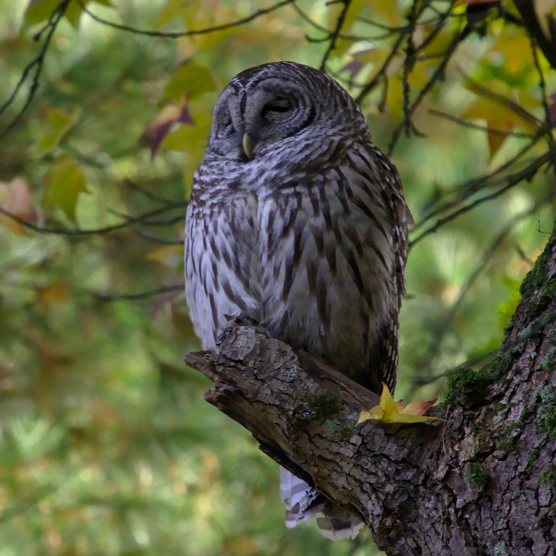
Save the following image as
~/cs2613/labs/L21/owl.jpg (make sure you get the full resolution image, and not the thumbnail).
Complete the following function using scale layers
function out = monochrome(in, weights=[0.21,0.72,0.07])
  out =
endfunction
Run the monochrome function on owl.jpg, you should get something like the following.
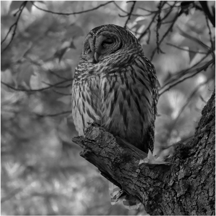
Try a few different values of weight vectors, see if you can generalize some rules from your experiments.
One useful operation on images is to detect how they are changing
locally. Roughly speaking the gradient can be thought about as
specifying both how much the intensity is changing, and what
direction that change is happening in. Octave returns that
information as an (x,y) vector using parallel arrays.
A = [0,0,0,0,0,1;
     0,1,1,1,0,0;
     0,1,1,1,0,1;
     0,1,1,1,1,0;
     0,1,1,1,1,0;
     0,0,0,0,0,0];

[Dx, Dy] = gradient(A);

imshow(A);
figure;
imshow(Dx);
figure;
imshow(Dy);
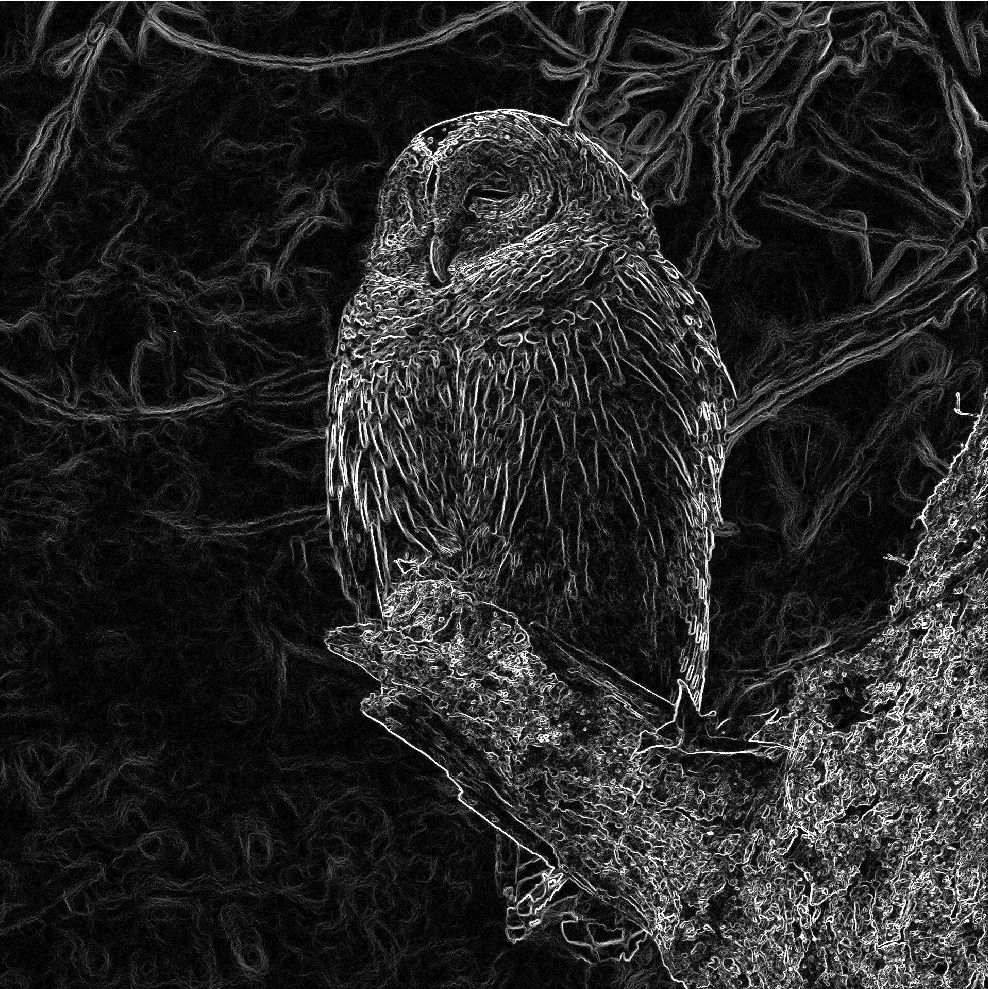
Complete the follow function, by combining the Dx and Dy arrays
into a single array such that normimg(i,j) = norm([Dx(i,j),Dy(i,j)]). Don't use a loop. The demo should produce an
image somewhat like the one below.
function normimg = normgrad(img)
  [Dx, Dy] = gradient(img);
  normimg =
endfunction

%!demo
%! owl=imread("owl.jpg");
%! monowl=monochrome(owl);
%! ng = normgrad(monowl);
%! imshow(ng*2, [0,20]);
One common feature of photo editing software (or camera firmware) is
to highlight overexposed or underexposed pixels. In this exercise we
will use our solutions for scale layers
(from L21) and monochrome in order to mark the pixels above
a certain level.
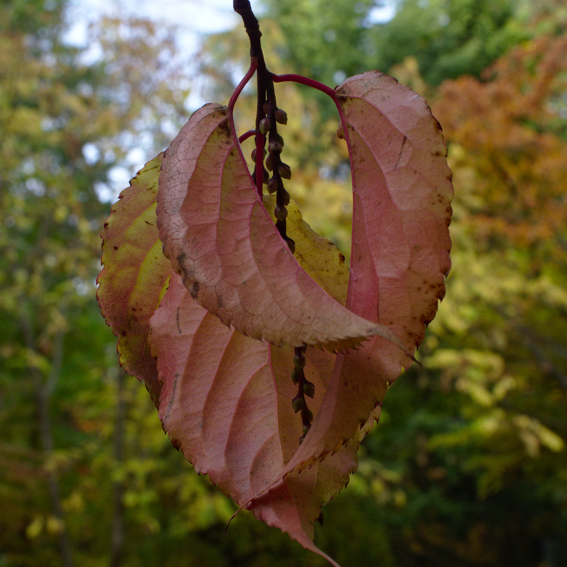
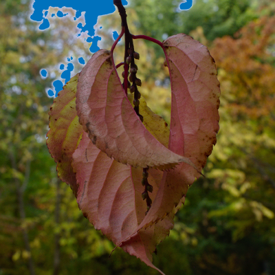
Download the following image (make sure you download the actual full
resolution image) and save it as ~/cs2613/labs/L22/leaf.jpg.
Use the builtin function find to complete the threshold function
to find all pixel positions with value higher than a given threshold.
Note that this use of find depends on broadcasting. In all
of the calls to plot in this lab, you may want to adjust
markersize to better see the selected pixels (it depends a bit on
screen resolution and image size).
function [rows, cols] = threshold(in, lower=100)
  [rows,cols] =
endfunction

%!test
%! A=[1,2,3; 4,5,6];
%!  [rows,cols]=threshold(A,4);
%!  assert(rows==[2;2]);
%!  assert(cols==[2;3]);

%!demo
%! leaf=imread("leaf.jpg");
%! monoleaf=monochrome(leaf);
%! [rows, cols] = threshold(monoleaf,200);
%! clf
%! hold on;
%! imshow(leaf);
%! plot(cols,rows,".","markersize",1);
The output of demo threshold should be something like the following.
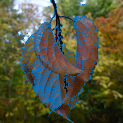
In order to extract a description of a scene from an image, an early
step is to detect the boundaries between various objects in the scene
via edge
detection. There are
many different methods, but one approach is to find pixels where the
gradient is particularly high. Use monochrome and normgrad
functions from above to complete the following script.
leaf=imread("leaf.jpg");
monoleaf=
ng =
[rows, cols] = threshold(ng, __ );

clf
hold on;
imshow(leaf);
plot(cols,rows,".","markersize",1);
Try different values for the threshold. The output of this script should be something like the following; it's interesting as far as detecting texture, but not very helpful for dividing the scene into objects. There's also a fair amount of isolated "edge" pixels in the background. Both of these problems can be addressed via smoothing in the next lab.
Read